Introduction

Recently, offline reinforcement learning methods have become widespread, which promises many prospects in solving problems of varying complexity. However, one of the main problems that researchers face is the optimism that can arise while learning. The agent optimizes its strategy based on the data from the training set and gains confidence in its actions. But the training set is quite often not able to cover the entire variety of possible states and transitions of the environment. In a stochastic environment, such confidence turns out to be not entirely justified. In such cases, the agent’s optimistic strategy may lead to increased risks and undesirable consequences.

In search of a solution to this problem, it is worth paying attention to research in the field of autonomous driving. It is obvious that the algorithms in this area are aimed at reducing risks (increasing user safety) and minimizing online training. One such method is SeParated Latent Trajectory Transformer (SPLT-Transformer) presented in the article “Addressing Optimism Bias in Sequence Modeling for Reinforcement Learning” (July 2022).

1. SPLT-Transformer method

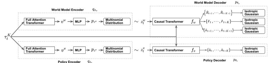
Similar to Decision Transformer, SPLT-Transformer is a sequence generation model using the Transformer architecture. But unlike the mentioned DT, it uses two separate information flows to model the Actor policy and the environment.

The method authors try to solve 2 main problems:

1. Models should help create a variety of candidates for the Agent’s behavior in any situation;
2. Models should cover most of the different modes of potential transitions to a new environment state.

To achieve this goal, we train 2 separate VAEs based on Transformer for Actor policy and environment model. The method authors generate stochastic latent variables for both flows and use them over the entire planning horizon. This allows us to enumerate all possible candidate trajectories without exponentially increasing branching and provides an effective search for behavior options during testing.

The idea is that latent policy variables should correspond to different high-level intentions, similar to the skills of hierarchical algorithms. At the same time, the latent variables of the environmental model should correspond to various possible trends and the most likely change in its state.

The policy and environmental encoders use the same architecture using Transformers. They receive the same initial data in the form of a previous trajectory. But unlike the previously discussed algorithms, the trajectory includes only a set of Actor states and actions. At the output of the encoders, we obtain discrete latent variables with a limited number of values in each dimension.

The authors of the method propose to use the average value of the transformer outputs for all elements in order to combine the entire trajectory into one vector representation.

Next, each of these outputs is processed by a small multilayer perceptron that outputs independent categorical distributions of the latent representation.

The policy decoder receives the same original trajectory as input, supplemented by the corresponding latent representation. The goal of a policy decoder is to estimate probabilities and predict the next most likely next action in a trajectory. The authors of the method present a decoder using the Transformer model.

As mentioned above, we remove the reward from the sequence, but add a latent representation. However, the latent representation does not replace the reward as a sequence element at each step. The method authors introduce a latent representation transformed by a single embedding vector similar to the positional encoding used in some other works using the Transformer architecture.

The environment model decoder has an architecture similar to the policy decoder. At the output only, the environmental model decoder has “three heads” to predict the most likely subsequent state and its cost, as well as the transition reward.

As in DT, models are trained on data from the training set using supervised learning methods. Models are trained to compare trajectories with subsequent actions (Actor), transitions to new states and their costs (environmental model).

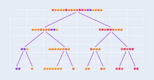
While testing and operation, the selection of the optimal action is carried out based on the assessment of candidate forecast trajectories at a given planning horizon. To compile one planned candidate trajectory, sequential generation of actions and states with rewards is carried out over the planning horizon. Then the optimal trajectory is selected and its first action is carried out. After the transition to a new state of the environment, the entire algorithm is repeated.

As you can see, the algorithm plans several candidate trajectories, but only one action of the optimal trajectory is performed. Although this approach may seem inefficient, it can minimize risks by planning several steps ahead. At the same time, it is possible to correct the trajectory in time as a result of re-evaluating each visited state.

The author’s visualization of the method is presented below.

2. Implementation using MQL5

After considering the theoretical aspects of the SPLT-Transformer method, let’s move on to implementing the proposed approaches using MQL5. I want to say right away that our implementation will be farther than ever from the author’s algorithm. The reason is my subjective perception. The entire experience of this series of articles demonstrates the complexity of creating an environmental model for financial markets. All our attempts yielded rather modest results. The accuracy of the forecasts is quite low at 1-2 steps. As the planning horizon grows, it tends to 0. Therefore, I decided not to build candidate trajectories, but to limit myself to only generating several candidate action options from the current state.

But this approach entails a gap between the action and its evaluation. As you can see in the visualization above, the Actor policy and the environmental model receive the same input data. But then the data flows in parallel streams. Therefore, when predicting the subsequent state and expected reward, the environmental model knows nothing about the action that the Agent will choose. Here we can only talk about a certain assumption with a certain degree of probability based on previous experience from the training sample. It should be noted that the training sample was created based on Actor policies different from those currently used one.

In the author’s version, this is leveled out by adding the Agent’s action and the forecast state to the trajectory at the next step. However, in our case, taking into account the experience of low quality planning for the subsequent state of the environment, we risk adding completely uncoordinated states and actions to the trajectory. This will lead to an even greater decrease in the quality of planning the next steps in the forecast trajectory. In my opinion, the efficiency of such planning and evaluation of such trajectories is very doubtful. Therefore, we will not waste resources on predicting candidate trajectories.

At the same time, we need a mechanism capable of comparing the Agent’s actions and the expected reward. On the one hand, we can use the Critic’s model, but this fundamentally breaks the algorithm and completely excludes the environmental model. Unless, of course, we use it as a Critic.

However, I decided to experiment with a different approach that is closer to the original algorithm. To begin with, I decided to use one encoder for both streams. The resulting latent state is added to the trajectory and fed to the input of 2 decoders. The actor, based on the initial data, generates a predictive action, and the environmental model returns the amount of the future discounted reward.

The idea is that, given the same input data, the models return consistent results. To do this, we exclude stochasticity in the Actor and environmental models. In doing so, we create stochasticity in the latent representation, which allows us to generate multiple candidate actions and associated predictive state estimates. Based on these estimates, we will rank candidate actions to select the optimal weighted step.

To optimize the number of operations performed, we should pay attention to one more point. By feeding the same trajectory to the Encoder input, we will repeat the results of all its internal layers with mathematical accuracy. Differences are formed only in the variational auto encoder layer when sampling from a given distribution. Therefore, to generate candidate actions, it is advisable for us to move the specified layer outside the Encoder. This will allow us to carry out only one Encoder pass at each iteration. After some thought, I moved the variational auto encoder layer into the environment model.

I went further along the path of optimizing the workflow. All three of our models use the same trajectory as input data. As you know, trajectory elements are not uniform. Before processing, they pass through an Embedding layer. This gave me the idea of embedding data in only one model, and then using the resulting data in the remaining two. Thus, I left the embedding layer only in the Encoder.

There is one more thing. The environment model and Actor use the concatenated vector of trajectory and latent representation as input. We have already determined that the variational auto encoder layer has been transferred to the environmental model for the formation of a stochastic latent representation. Here we will carry out the combination of vectors and pass the already obtained result to the Actor’s input.

Now let’s transfer the above ideas into the code. Let’s create a description of our models. As always, it is formed in the CreateDescriptions method. In the parameters, the method receives pointers to three objects describing our models.